Matrix factorization is the process of reversing matrix multiplication. Well not technically, but matrix factorization searches for factor matrices which, when multiplied together, approximate the original data matrix. It turns out that these factors contain insights into the underlying trends of the data. For example, if the data matrix contains movie ratings, the resultant factors may represent movie genre/category and the genre preferences of movie watchers, respectively. This insight can then be used to identify common groups or patterns in the data and, combined with other auxiliary methods, make recommendations to users. As a result, matrix factorization is a useful tool in recommender systems and collaborative filtering. To simplify things, we’ll focus on the model with exactly two factors.
Model Setup
We aim to solve the matrix factorization equation
\begin{align} X \approx AS \end{align}
where \(X \in \mathbb{R}^{m \times n}\) is the data matrix and \(A \in \mathbb{R}^{m \times k}\) and \(S \in \mathbb{R}^{k \times n}\) are the left and right factors, respectively. Here, \(k\) is the “factor rank”, or the rank of the approximation computed. While there is no correct determination of the factor rank, it can be determined through testing or heuristics and is ideally less than \(m\) and \(n\) to reduce dimensionality. We use “approximately” rather than “equal” because solving this equation is actually quite difficult. Just like how an integer can have many possible factorizations (\(64\) can be factored into \(8 \times 8\) or \(16 \times 4\)), matrices have many possible factorizations as well. In fact, an exact approximation is exceptionally rare, especially when the dimensions of a matrix increase. Thus, finding a solution to this equation is effectively identical to minimizing
\begin{align} min \quad ||X - AS||_F^2 \end{align}
where \(||\cdot||_F\) is the Frobenius norm. Note that finding a global minimum is often intractable, leaving a local minimum to be the more realistic solution. Because we are solving for both \(A\) and \(S\) simultaneously, gradient calculation methods won’t work. Instead, we turn to other means, a straightforward choice of which is alternating least squares (ALS).
Alternating Least Squares (ALS)
As the name suggests, ALS alternates between the two factors and performs several computations. First, it randomly initializes \(A\) and \(S\). Then, it randomly selects a column of the data matrix (or a row of the data matrix) to form the equations
\begin{align} A y \approx X_{:,i} \text{ or } z^T S \approx X_{j,:} \end{align}
where the subscript \(:\) represents all rows/columns of a matrix. These equations(which are linear systems) now have solutions which can be found using the method of least squares. In particular, it solves for \(y\)(or \(z^T\)) using the normal equations. Finally, it replaces the corresponding column of \(S\)(or row of \(A\)) with the least squares solution, that is
\begin{align} S_{:,i} := (A^T A)^{-1}A^T X_{:, i} \text{ or } A_{j,:} <- (S S^T)^{-1} S X_{j,:}^T \end{align}
This process is then repeated for a specified number of iterations or until the error measure is sufficiently small(a useful measure is relative error).
Implementation
We first turn our attention to computing the least squares solution. While outright computing \((A^T A)^{-1}A^T y\) is certainly an option, it isn’t ideal for inconsistent systems which can cause numerical errors. Instead, using the np.linalg.lstsq() function is more reliable in most scenarios (for a comparison between np.linalg.solve() and lstsq() see this helpful stackoverflow post. Note that we only need to consider the case where the right factor is updated since we can simply transpose the equation for the left factor.
	import numpy as np

	def lstupdate(A, S, X, ind):
		lstsol = np.linalg.lstsq(A, X[:, ind], rcond = None)[0]
		return lstsol
Initializing the factors can be done simply by randomly generating matrices with the correct dimensions(or taking pre-initialized factors from the user). Alternating between the two factors is simple as well. We just need to randomly sample a row/column and update it using the ALS update.
	def als(X, k, it, **kwargs):
		num_row, num_col = X.shape
		A = kwargs.get("A", np.random.rand(num_row, k))
		S = kwargs.get("S", np.random.rand(k, num_col))

		row_ind = np.arange(num_row)
		col_ind = np.arange(num_col)
		for i in range(it):
			col = np.random.choice(col_ind, size = 1)
			S[:, col] = lstupdate(A, S, X, col)
			row = np.random.choice(row_ind, size = 1)
			A[row, :] = lstupdate(S.T, A.T, X.T, row).T
		return(A, S)
To evaluate the performance of the algorithm, we need an error measure to gauge the quality of the approximation. One useful measure is relative error, or the ratio of absolute error to the ground truth measurement. In this case, it can be computed using the following formula:
\begin{align} \epsilon = \frac{|AS - X|_F^2}{|X|_F^2} \end{align}
	def relerror(A, S, X):
		return np.linalg.norm(X - A @ S) / np.linalg.norm(X)
Testing
Next, we’ll explore how varying the parameters can affect the resulting approximation. As of now, we can vary the number of iterations, factor rank, and number of iterations. A useful way to get started is to test with a generative model, where the synthetic data matrix is created by multiplying pre-determined factors. This ensures there is indeed a perfect factorization for the algorithm to aim for (and provides a much needed sanity check as well).
Looking first at the number of iterations, we can run ALS on a small generated data matrix with varying iterations and plot the corresponding relative errors.
	import matplotlib.pyplot as plt

	np.random.seed(18)
	A = np.random.rand(200,80)
	S = np.random.rand(80,80)
	X = A @ S

	its = [1, 10, 100, 1000, 3000]
	errs = [-1, -1, -1, -1, -1]
	for ind, it in enumerate(its):
		approxA, approxS = als(X, 5, it)
		errs[ind] = relerror(approxA, approxS, X)

	plt.plot(its, errs)
	plt.ylim(0, 1)
	plt.xlabel("number of iterations")
	plt.ylabel("relative error")
	plt.show()
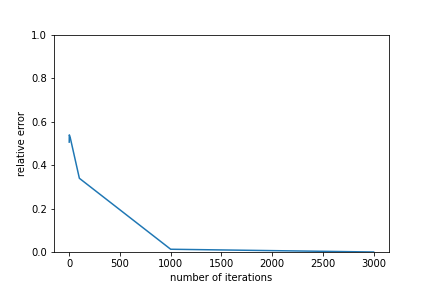
Predictably, increasing the number of iterations lowers the relative error(and increases the approximation quality). However, after a certain threshold the improvements diminish significantly, indicating that the algorithm may have reached a local minimum. For this reason, it may be worthwhile to add a second exit condition that stops the ALS algorithm when relative error reductions fall below a certain point.
Of course, bigger datasets will require more iterations to reach a local minimum. Alongside this, there is a second scaling issue: the increasing computation required for a single ALS iteration. We can observe this by taking the average of \(100\) iterations and increasing the size of the generated data matrix.
	import time

	np.random.seed(188)

	dims = [1000*x for x in range(1, 11)]
	times = [-1 for d in dims]
	for ind, dim in enumerate(dims):
		A = np.random.rand(dim, 5)
		S = np.random.rand(5, dim)
		X = A @ S

		start = time.time()
		approxA, approxS = als(X, 5, 1000)
		end = time.time()

		times[ind] = (end - start)

	plt.plot(dims, times)
	plt.xlabel("number of iterations")
	plt.ylabel("runtime (secs)")
	plt.show()
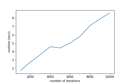
As the amount of data increases, the amount of time required for ALS to run also increases. While the numbers here don’t seem like a big deal, the runtime can scale quickly as datasets grow larger and larger(\(10000\) is a puny dataset by some standards) as well as with a larger factor rank. So while ALS is quick to converge, it can be increasingly expensive to utilize in many practical applications.
Finally, we can observe how the factor rank affects the approximation quality. So far, we’ve been picking the correct factor rank to ensure the relative error can approach zero(the generative model allows us to cheat). However, factor ranks that are rather far from the true rank can cause the relative error to plateau.
	np.random.seed(1888)
	A = np.random.rand(2000,50)
	S = np.random.rand(50,800)
	X = A @ S

	ks = [10, 20, 30, 40, 50, 60, 70, 80, 90, 100]
	errs = [-1 for x in range(len(ks))]
	for ind, k in enumerate(ks):
		approxA, approxS = als(X, k, 2000)
		errs[ind] = relerror(approxA, approxS, X)

	plt.plot(ks, errs)
	plt.xlabel("factor rank")
	plt.ylabel("relative error after 2000 iterations")
	plt.show()
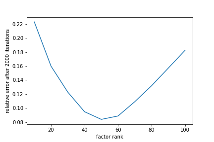
It is apparent that the lowest relative error occurs when the factor rank matches the true rank of the data matrix while substantially smaller or larger factor ranks cause the relative error to stall much earlier. While inconvenient, picking an accurate factor rank may not always be meaningful, however. Matrix factorization is useful for dimension reduction, so forcing the factor rank to be lower makes sense in many applications.
Other Algorithmic Additions
There are yet more features we can include in the matrix factorization framework. For instance, one could perform each row/column update more than once after sampling. This could speed up the rate of convergence, but may also introduce issues with oversolving certain portions of the factor matrices. One could also alter the sampling method - rather than uniformly selecting a row/column, a weighted sampling method could be used instead. While this could also speed up convergence by targeting more imbalanced rows/columns, calculating the probabilities requires yet more computation(which may or may not be worth the benefit).
Conclusion
Alternating least squares is a powerful method to factorize matrices and uncover latent topics. However, the computational power and runtime scales quickly with the amount of data and increases the runtime needed to compute a decent approximation. These drawbacks can be mitigated by substituting the least squares method of solving linear systems with a different solver. One such solver is the Kaczmarz method, which estimates the least squares solution. Check out this preprint for more information on a Kaczmarz-based matrix factorization algorithm.