Bayesian Regression

Bayesian Linear Regression

In this notebook, we explore linear regression under the Bayesian framework. While traditional or frequentist linear regression treats the model parameters(such as the slope and intercept) as deterministic, Bayesian linear regression assumes that these parameters come from a hidden or latent probability distribution. The Bayesian framework has the clear benefit of incorporating prior domain knowledge an individual may have on a given dataset or application. Furthermore, a Bayesian treatment of regression can also help avoid overfitted or overly-complex models, issues that often plague frequentist maximum likelihood methods [Bishop 152]. Let’s start with a quick rundown of traditional linear regression. Both the IPython notebook and code are available.

Notation

We will denote constants as lower case letters \(a\), vectors as lower case letters with a vector symbol \(\vec{a}\), and matrices as upper case bolded letters \(\mathbf{A}\).

Frequentist Treatment

Suppose our data consists of i.i.d. target/response variables \(t_i\) and corresponding predictor/explanatory variables $\vec{x_i} = (x_{i,0}, x_{i,1}, \ldots, x_{i,N-1})$. Rather than using the original data, it is common to instead use extracted/preprocessed features(see monomial basis and RBF for examples), which we will denote \(\vec{\phi_i} = \left(\phi_0(\vec{x_i}), \phi_1(\vec{x_i}), \ldots, \phi_{M-1}(\vec{x_i})\right)\). We then assume that \(t_i\) has a linear relationship with \(\vec{\phi_i}\). Adding random noise \(\epsilon_i\), we have

where \(\vec{w} = (w_0, w_1, \ldots, w_{N-1})\) are our model parameters/coefficients.

In the case of simple linear regression,

It is also common to assume that the random noise \(\epsilon_i\) comes from a Gaussian distribution with zero mean and inverse variance(precision) \(\beta\),

	# simple linear regression with no basis function for simplicity and sake of visualization
	import numpy as np
	import matplotlib.pyplot as plt
	np.random.seed(1)

	dim = 1
	# generate toy data
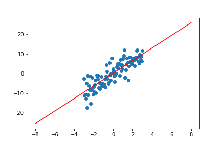
	numpoints = 100
	x = np.linspace(-3, 3, numpoints)
	x = x[np.newaxis].T

	slope = 3
	eps_mu = 0
	beta = 0.25
	eps = np.random.normal(eps_mu, 1/beta, size = (numpoints, dim))
	t = slope * x + eps

	# phi is a column of ones next to the column of x's
	phi = np.hstack((np.ones((numpoints, 1)), x))

Because adding a constant to a Gaussian distribution shifts the mean by that constant, we have

We can then write the likelihood function and log-likelihood function as a product of the individual likelihoods/log-likelihoods due to independence

Maximizing the log-likelihood is the same as minimizing the likelihood, so taking the gradient with respect to \(\vec{w}\) and setting to zero yields the famous normal equations,

where \(\mathbf{\Phi} = \left(\vec{\phi_0}, \vec{\phi_1}, \ldots, \vec{\phi_N}\right)^T\) is often referred to as the design matrix.

	# pinv is generally avoided since singular matrices can cause problems
	#w = np.linalg.pinv(phi.T @ phi) @ phi.T @ t

	# use lstsq instead, it solves for x in Ax = b
	w = np.linalg.lstsq(phi.T @ phi, phi.T @ t, rcond=None)[0]

	# plot data and fitted reg. line
	line_x_ls = np.linspace(np.min(x)-5, np.max(x) + 5, 100)
	line_y_ls = w[0] + w[1]*line_x_ls
	plt.scatter(x, t)
	plt.plot(line_x_ls, line_y_ls, 'r')
	plt.show()

Bayesian Treatment

Bayesian linear regression follows the same setup as the frequentist framework, except that we now assume that \(\vec{w}\) belongs to a prior distribution. It turns out that because the likelihood function \(L(\vec{w})\) is the exponential of a quadratic function of \(\vec{w}\), this prior is a multivariate Gaussian distribution [Bishop 152]

where \(\vec{m_0}\) and \(\mathbf{S}_0\) are the initial “guesses” of the mean and covariance of \(\vec{w}\). The posterior distribution of \(\vec{w}\) can then be found using Baye’s Rule,

Note that \(p(\vec{t} | \vec{w})\) is the likelihood given in the previous section (since we view \(\vec{x}\) and \(\beta\) as constant). The posterior distribution of a Gaussian will in turn be Gaussian, and given the prior and likelihood distributions [Bishop 90-93]

the posterior distribution will have the following form [Bishop 93]

This works out to be

Rather than maximizing the likelihood, we instead maximize the posterior, or maximum a posteriori(MAP) (which is actually equivalent to MLE if the prior is constant or uniform). In the case of a Gaussian posterior distribution, the mode coincides with the mean, thus

For the skeptical, we can also compute this directly. Recall that $w \in \mathbb{R}^M$, thus

	# choose an uninformative prior for simplicity
	m_0 = np.array([[0], [0]])
	S_0 = np.eye(2)
	beta = 0.25

	S_0inv = np.linalg.lstsq(S_0, np.eye(2), rcond = None)[0]
	S_n = np.linalg.lstsq(S_0inv + beta * phi.T @ phi, np.eye(2), rcond = None)[0]
	m_n = S_n @ (S_0inv @ m_0 + beta * phi.T @ t)

	line_x_b = np.linspace(np.min(x)-5, np.max(x) + 5, 100)
	line_y_b = m_n[0] + m_n[1]*line_x_b

	fig, ax = plt.subplots(1,2, figsize=(10,5))
	ax[0].title.set_text("Least Squares")
	ax[0].scatter(x, t)
	ax[0].plot(line_x_ls, line_y_ls, 'r')
	ax[1].title.set_text("Bayesian")
	ax[1].scatter(x, t)
	ax[1].plot(line_x_b, line_y_b, 'r')
	plt.show()

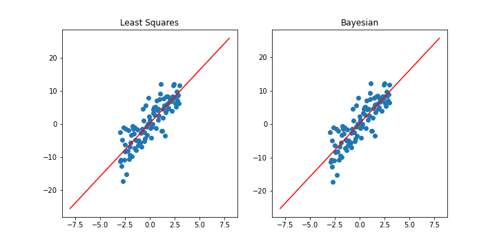
The fitted Bayesian model is almost identical to the frequentist model in this simple regression case. This is because we considered a zero-mean isotropic prior(where \(m_0 = 0\) and \(S_0 = \alpha^{-1} I\) for some constant \(\alpha\)), thus maximizing the log-posterior yields an identical solution to that of MLE(with an added regularization term). In other words, if our prior for \(\vec{w}\) is uninformative, Bayesian regression reduces to frequentist regression. We will explore this idea further after a quick detour to an online version of Bayesian regression.

Regularization

As previously mentioned, a zero-mean isotropic prior leads to a maximum a posteriori solution identical to the MLE solution for regularized frequentist regression(specifically ridge regression). We can see this by direct computation of the log posterior. Rather than recomputing the posterior, we can simply add the log likelihood(same likelihood as the frequentist version) and log prior.
Recall that the prior and log prior are

Thus the log posterior is

The log posterior is identical to the loss function for ridge regression with \(\lambda = \frac{\alpha}{\beta}\), and minimizing it will yield the same solution to ridge regression. Because a larger \(\alpha\) reflects a stronger belief in the prior, a large \(\alpha\) will result in regularization. However, this is double-edged: a strong belief in an incorrect prior can lead to misleading results or worse fits. We can demonstrate this regularizing effect in the following example of a \(4\)-dimensional polynomial.

	import numpy as np
	import matplotlib.pyplot as plt
	np.random.seed(1)

	# generate toy data
	dim = 1
	numpoints = 100
	x = np.linspace(-3, 3, numpoints)
	x = x[np.newaxis].T

	eps_mu = 4
	beta = 0.125
	eps = np.random.normal(eps_mu, 1/beta, size = (dim, numpoints)).T
	t = 0.5 * x**4 + eps

	# phi is 5 columns of x^i for i in {0, 1,... 4}
	phi = np.hstack((np.ones((numpoints, 1)), x, x**2, x**3, x**4))

	# use lstsq instead, it solves for x in Ax = b
	w = np.linalg.lstsq(phi.T @ phi, phi.T @ t, rcond=None)[0]
	print("frequentist:", w.T)
	# draw fitted polynomial
	line_x_ls = np.linspace(np.min(x), np.max(x), 100)
	line_y_ls = w[0] + w[1]*line_x_ls + w[2]*line_x_ls**2 + w[3]*line_x_ls**3 + w[4]*line_x_ls**4 

	# zero-mean isotropic prior with alpha = 10
	m_0 = np.array([[0], [0], [0], [0], [0]])
	S_0 = 0.1 * np.eye(5)
	beta = 0.125

	# calculate bayesian params
	S_0inv = np.linalg.lstsq(S_0, np.eye(5), rcond = None)[0]
	S_n = np.linalg.lstsq(S_0inv + beta * phi.T @ phi, np.eye(5), rcond = None)[0]
	m_n = S_n @ (S_0inv @ m_0 + beta * phi.T @ t)
	# draw bayesian fitted polynomial
	line_x_b = np.linspace(np.min(x), np.max(x), 100)
	line_y_b = m_n[0] + m_n[1]*line_x_b + m_n[2]*line_x_b**2 + m_n[3]*line_x_b**3 + m_n[4]*line_x_b**4 
	print("Bayesian:   ", m_n.T)

	fig, ax = plt.subplots(1,2, figsize=(10,5))
	ax[0].title.set_text("Least Squares")
	ax[0].scatter(x, t)
	ax[0].plot(line_x_ls, line_y_ls, 'r')
	ax[1].title.set_text("Bayesian")
	ax[1].scatter(x, t)
	ax[1].plot(line_x_b, line_y_b, 'r')
	plt.show()

\(\begin{align} \text{frequentist}: &[[ 5.56943855, 1.14653262, -0.76132086, -0.12806114, 0.57386762]]\newline \text{Bayesian}: &[[ 1.73468395, 0.43333639, 0.77427287, -0.01914878, 0.44023857]] \end{align}\)

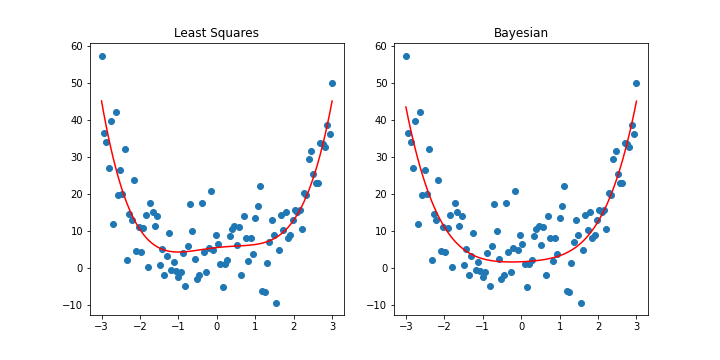
With a relatively strong prior, we can see that the Bayesian model penalizes large coefficients and leads to a relatively simpler model than the frequentist one. We would see a similar effect if we applied ridge regression with \(\lambda = 40\).

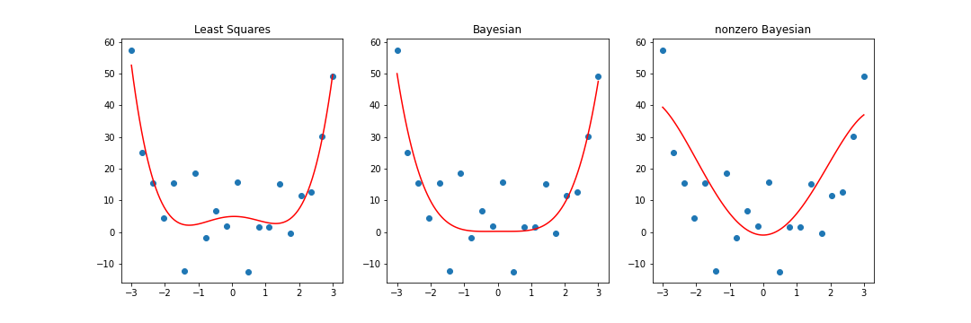
However, this is all with a prior mean of \(0\). If we consider a non-zero mean, we could attempt to nudge the Bayesian coefficients in a certain direction. Although this effect would most likely be lost with the addition of more data, it is more pronounced during early stages of training when there is fewer data available. Consider the case with the first \(n = 20\) observations rather than the full \(n = 100\). We may have reason to believe that the data follows a parabolic shape(a \(2\) degree polynomial looks similar to a \(4\) degree polynomial after all). Setting the prior for the second degree coefficient to be nonzero, we end up something different.

	import numpy as np
	import matplotlib.pyplot as plt
	np.random.seed(1)

	# generate toy data
	numpoints = 20
	x = np.linspace(-3, 3, numpoints)
	x = x[np.newaxis].T

	eps_mu = 4
	beta = 0.125
	eps = np.random.normal(eps_mu, 1/beta, size = (dim, numpoints)).T
	t = 0.5 * x**4 + eps

	# phi is 5 columns of x^i for i in {0, 1,... 4}
	phi = np.hstack((np.ones((numpoints, 1)), x, x**2, x**3, x**4))

	# use lstsq instead, it solves for x in Ax = b
	w = np.linalg.lstsq(phi.T @ phi, phi.T @ t, rcond=None)[0]
	print("frequentist:        ", w.T)
	# draw fitted polynomial
	line_x_ls = np.linspace(np.min(x), np.max(x), 100)
	line_y_ls = w[0] + w[1]*line_x_ls + w[2]*line_x_ls**2 + w[3]*line_x_ls**3 + w[4]*line_x_ls**4 

	# zero-mean isotropic prior with alpha = 10
	m_0 = np.array([[0], [0], [0], [0], [0]])
	S_0 = 0.1 * np.eye(5)
	beta = 0.125

	# calculate bayesian params
	S_0inv = np.linalg.lstsq(S_0, np.eye(5), rcond = None)[0]
	S_n = np.linalg.lstsq(S_0inv + beta * phi.T @ phi, np.eye(5), rcond = None)[0]
	m_n = S_n @ (S_0inv @ m_0 + beta * phi.T @ t)
	# draw bayesian fitted polynomial
	line_x_b1 = np.linspace(np.min(x), np.max(x), 100)
	line_y_b1 = m_n[0] + m_n[1]*line_x_b + m_n[2]*line_x_b**2 + m_n[3]*line_x_b**3 + m_n[4]*line_x_b**4 
	print("Bayesian:           ", m_n.T)

	# nonzero-mean isotropic prior with alpha = 10
	m_0 = np.array([[0], [0], [10], [0], [0]])
	S_0 = 0.1 * np.eye(5)
	beta = 0.125

	# calculate bayesian params
	S_0inv = np.linalg.lstsq(S_0, np.eye(5), rcond = None)[0]
	S_n = np.linalg.lstsq(S_0inv + beta * phi.T @ phi, np.eye(5), rcond = None)[0]
	m_n = S_n @ (S_0inv @ m_0 + beta * phi.T @ t)
	# draw bayesian fitted polynomial
	line_x_b2 = np.linspace(np.min(x), np.max(x), 100)
	line_y_b2 = m_n[0] + m_n[1]*line_x_b + m_n[2]*line_x_b**2 + m_n[3]*line_x_b**3 + m_n[4]*line_x_b**4 
	print("nonzero Bayesian:   ", m_n.T)

	fig, ax = plt.subplots(1,3, figsize=(15,5))
	ax[0].title.set_text("Least Squares")
	ax[0].scatter(x, t)
	ax[0].plot(line_x_ls, line_y_ls, 'r')
	ax[1].title.set_text("Bayesian")
	ax[1].scatter(x, t)
	ax[1].plot(line_x_b1, line_y_b1, 'r')
	ax[2].title.set_text("nonzero Bayesian")
	ax[2].scatter(x, t)
	ax[2].plot(line_x_b2, line_y_b2, 'r')
	plt.show()